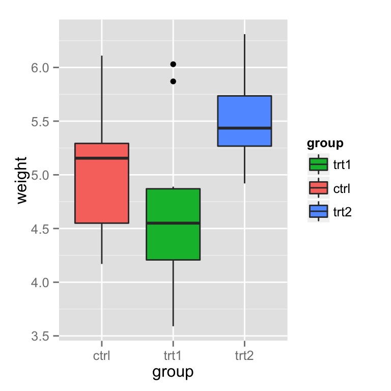
library(ggplot2)
bp <- ggplot(data=PlantGrowth, aes(x=group, y=weight, fill=group)) + geom_boxplot()
Use guides(fill=FALSE), replacing fill with the desired aesthetic. 使用 guides(fill=FALSE) 移除由ase中 匹配的fill生成的图例, 也可以使用theme You can also remove all the legends in a graph, using theme.
bp + guides(fill=FALSE)
bp + scale_fill_discrete(guide=FALSE)
bp + theme(legend.position="none")
修改图例的内容
改变图例的顺序为 trt1, ctrl, trt2:
bp + scale_fill_discrete(breaks=c("trt1","ctrl","trt2"))
 根据不同的分类,可以使用
 scale_fill_manual, scale_colour_hue,scale_colour_manual, scale_shape_discrete, scale_linetype_discrete 等等.
颠倒图例的顺序
bp + guides(fill = guide_legend(reverse=TRUE))
bp + scale_fill_discrete(guide = guide_legend(reverse=TRUE))
bp + scale_fill_discrete(breaks = rev(levels(PlantGrowth$group)))
隐藏图例标题
bp + guides
(fill=guide_legend(title=NULL))
bp + theme(legend.title=element_blank())
修改图例中的标签
两种方法一种是直接修改标签, 另一种是修改data.frame
Using scales
图例可以根据 fill, colour, linetype, shape 等绘制, 我们以 fill 为例, scale_fill_xxx, xxx 表示处理数据的一种方法, 可以是 hue(对颜色的定量操作), continuous(连续型数据处理), discete(离散型数据处理)等等.
bp + scale_fill_discrete(name="Experimental\nCondition")
bp + scale_fill_discrete(name="Experimental\nCondition",
breaks=c("ctrl", "trt1", "trt2"),
labels=c("Control", "Treatment 1", "Treatment 2"))
bp + scale_fill_manual(values=c("#999999", "#E69F00", "#56B4E9"),
name="Experimental\nCondition",
breaks=c("ctrl", "trt1", "trt2"),
labels=c("Control", "Treatment 1", "Treatment 2"))
注意这里并不能修改 x轴 的标签,如果需要改变x轴的标签,可以参照http://blog.csdn.net/tanzuozhev/article/details/51107583
df1 <- data.frame(
sex = factor(c("Female","Female","Male","Male")),
time = factor(c("Lunch","Dinner","Lunch","Dinner"), levels=c("Lunch","Dinner")),
total_bill = c(13.53, 16.81, 16.24, 17.42)
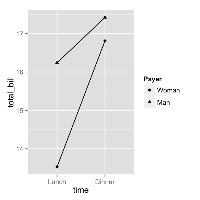
lp <- ggplot(data=df1, aes(x=time, y=total_bill, group=sex, shape=sex))
+ geom_line() + geom_point()
lp + scale_shape_discrete(name ="Payer",
breaks=c("Female", "Male"),
labels=c("Woman", "Man"))
 If you use both colour and shape, they both need to be given scale specifications. Otherwise there will be two two separate legends. 如果同时使用
 color和shape,那么必须都进行scale_xx_xxx的定义,否则color和shape的图例就会合并到一起, 如果 scale_xx_xxx 中的name相同,那么他们也会合并到一起.
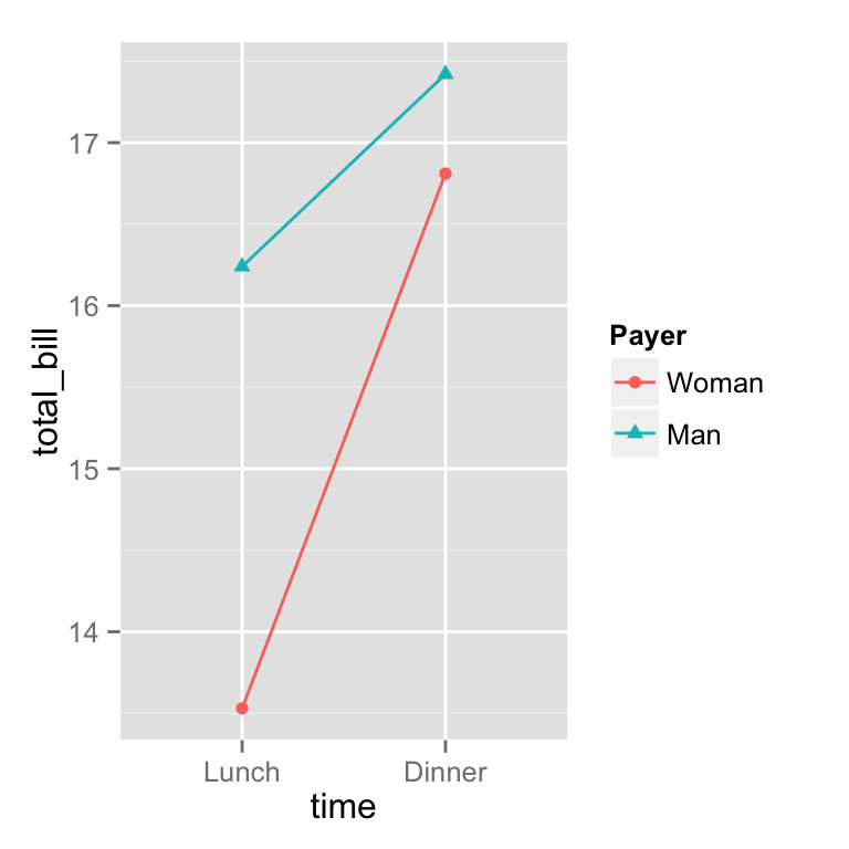
lp1 <- ggplot(data=df1, aes(x=time, y=total_bill, group=sex, shape=sex, colour=sex)) + geom_line() + geom_point()
lp1 + scale_colour_discrete(name ="Payer",
breaks=c("Female", "Male"),
labels=c("Woman", "Man"))
lp1 + scale_colour_discrete(name ="Payer",
breaks=c("Female", "Male"),
labels=c("Woman", "Man")) +
scale_shape_discrete(name ="Payer",
breaks=c("Female", "Male"),
labels=c("Woman", "Man"))
 ### scale的种类
scale_xxx_yyy:
xxx 的分类 colour: 点 线 或者其他图形的框线颜色 fill: 填充颜色 linetype :线型, 实线 虚线 点线 shape: 点的性状,超级多,可以自己搜索一下 size: 点的大小 alpha: 透明度
yyy 的分离 hue: 设置色调范围(h)、饱和度(c)和亮度(l)获取颜色 manual: 手动设置 gradient: 颜色梯度 grey: 设置灰度值discrete: 离散数据 (e.g., colors, point shapes, line types, point sizes) continuous 连续行数据 (e.g., alpha, colors, point sizes)
修改data.frame的factor
pg <- PlantGrowth
levels(pg$group)[levels(pg$group)=="ctrl"] <- "Control"
levels(pg$group)[levels(pg$group)=="trt1"] <- "Treatment 1"
levels(pg$group)[levels(pg$group)=="trt2"] <- "Treatment 2"
names(pg)[names(pg)=="group"] <- "Experimental Condition"
head(pg)
## weight Experimental Condition
## 1 4.17 Control
## 2 5.58 Control
## 3 5.18 Control
## 4 6.11 Control
## 5 4.50 Control
## 6 4.61 Control
ggplot(data=pg, aes(x=`Experimental Condition`, y=weight, fill=`Experimental Condition`)) +
geom_boxplot()
修改标题和标签的显示
bp + theme(legend.title = element_text(colour="blue", size=16, face="bold"))
bp + theme(legend.text = element_text(colour="blue", size = 16, face = "bold"))
修改图例的框架
bp + theme(legend.background = element_rect())
bp + theme(legend.background = element_rect(fill="gray90", size=.5, linetype="dotted"))
设置图例的位置
图例的位置(left/right/top/bottom):
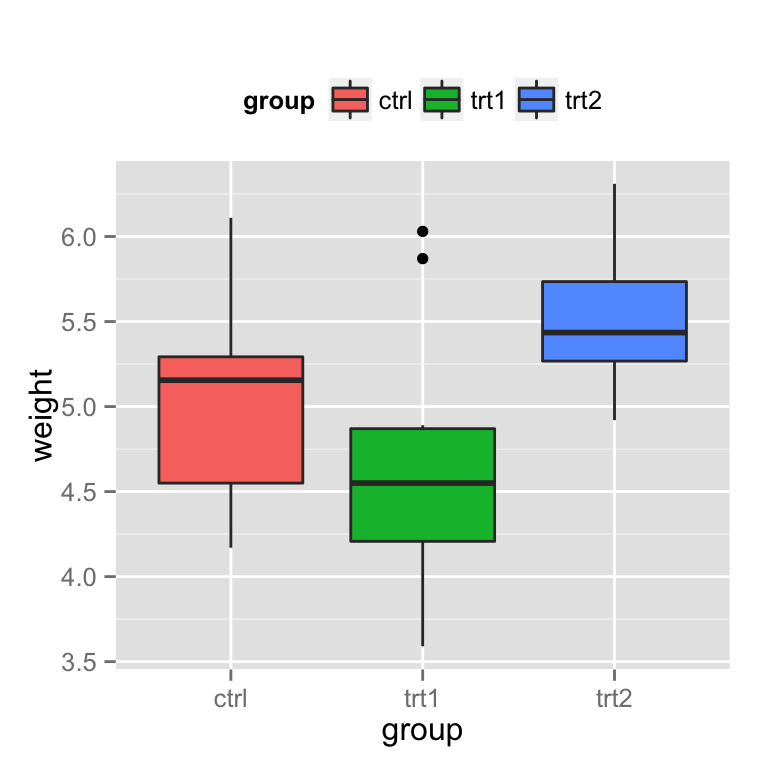
bp + theme(legend.position="top")
 也可以根据坐标来设置图例的位置, 左下角为 (0,0), 右上角为(1,1)
bp + theme(legend.position=c(.5, .5))
bp + theme(legend.justification=c(0,0),
legend.position=c(0,0))
bp + theme(legend.justification=c(1,0), legend.position=c(1,0))
ggplot(data=PlantGrowth, aes(x=group, fill=group)) +
geom_bar()
ggplot(data=PlantGrowth, aes(x=group, fill=group)) +
geom_bar(colour="black")
ggplot(data=PlantGrowth, aes(x=group, fill=group)) +
geom_bar() +
geom_bar(colour="black", show_guide=FALSE)
本文更新地址:http://blog.csdn.net/tanzuozhev/article/details/51106909本文在 http://www.cookbook-r.com/Graphs/Scatterplots_(ggplot2)/ 的基础上加入了自己的理解图例用来解释图中的各种含义,比如颜色,形状,大小等等, 在ggplot2中aes中的参数(x, y 除外)基本都会生成图例来解释
可以使用ggplot2的labs函数来修改图例的名称。例如:
ggplot(data, aes(x = x, y = y, color = group)) +
geom_point() +
labs(color = "图例的名称")
你也可以使用theme函数来修改图例的样式,例如:
ggplot(data, aes(x = x, y = y, color = group)) +
* @Date: 2019-11-19 18:44:04
* @LastEditTime: 2020-02-19 16:40:48
* @LastEditors: Please set LastEditors
import React from 'rea...
import React, { useState, useEffect, useRef} from "react";
import "./chart.less"
import { Chart } from "@antv/
g2";
const Charts = () => {
const chartRef = useRef()
const data = [
{ name: "杭州银行", score: 2, num: 5, city: "bj" },
引言图例的设置包括移除图例、改变图例的位置、改变标签的顺序、改变图例的标题等。移除图例有时候你想移除图例,使用 guides()。library(ggplot2)
p <- ggplot(PlantGrowth, aes(x=group, y=weight, fill=group)) + geom_boxplot()
p + guides(fill=FALSE)改变图例的位置我们可以用theme(l
此文内容首发于微信公众号:R语言搬运工,关注公众号浏览更多精彩内容\color{blue}{此文内容首发于微信公众号:R语言搬运工,关注公众号浏览更多精彩内容}此文内容首发于微信公众号:R语言搬运工,关注公众号浏览更多精彩内容
文末二维码
交流分享扣扣群:925920448\color{red}{交流分享扣扣群:925920448}交流分享扣扣群:925920448
使用ggplot2绘制统计图的时候,经常需要根据个人需要调整参数,使图例能够符合个人的审美。ggplot2的一个优点就是为我们提供了丰富的
itemCfg
图例子项配置信息
layout 布局方式 horizontal,vertical,默认 horizontal
align 位置,top,left,right,bottom
checkable 子选项是否可以触发checked 操作,默认所有的选项都是勾选
leaveChecked 是否保留一项不能取消勾选,默认为false
back
图例外边框和背景的配置信息,是一个矩形,参考
spacingX 子项之间的间距,x轴方向
spacingY
ggplot(raw_em, aes(x=ymd(date))) +
#color添加到aes()中,color = ‘legend里显示的分类名称’
geom_line(aes(y = PM2_5/1000,color="PM2.5"),size = 0.5) +
geom_line(aes(y = NOx/10^5,color= 'NOx'),size = 0.5)+
geom_line(aes(y = HC/1000,color= 'HC'),size = 0.5)+
geom.

