|
|
|

机器学习中有哪些涉及统计因果推断的算法?
机器学习分析数据似乎强调利用数据之间的相关关系进行预测,想知道是否有些算法设计因果推断的理论?
关注者
82
被浏览
50,933
7 个回答

这里介绍下微软开发的 DoWhy框架和因果森林(EconML包),其核心算法是 Double Machine Learning。以下提供了一个官方案例进行具体说明。
DoWhy 的作用:
- 建立因果模型(LinearDML)(DML: LinearDL, CausalForestDML)
- 识别影响效果(LinearDML.dowhy.fit(): Backdoor,Frontdoor,IV)
- 检验因果假设 - 稳健性检验(添加随机共同原因变量、安慰剂检验、随机删除部分样本)
EconML DML 估计器的作用:
- 考虑干预的变动
- 分析影响的异质性
- EconML CATE SingleTreeCateInterpreter -- 展示各个 features 的作用大
- EconML CATE SingleTreePolicyInterpreter -- 提出最优政策方案,即指出具体的细分样本+干预方案,以达到收益最大
本例中的最优政策方案:指出具体的细分顾客群体,对应的折扣方案,及对应的总收益(考虑折扣带来的成本)
案例说明: 找出最优的促销方案,决定给不同收入水平的顾客,提供不同的折扣方案,以达到利润最大化。
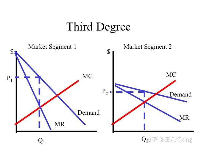

btw,三级价格歧视的极端情况下,是为每一个消费者制定一个ta最高能接受的价格,以实现利润最大化。
1. 数据准备
## 准备工作
import warnings
warnings.simplefilter('ignore')
import os
import urllib.request
import numpy as np
import pandas as pd
from networkx.drawing.nx_pydot import to_pydot
from IPython.display import Image, display
## 导入机器学习包的相关工具
from sklearn.preprocessing import PolynomialFeatures
from sklearn.ensemble import GradientBoostingRegressor
## 导入 EconML 包的相关工具
from econml.dml import LinearDML, CausalForestDML
from econml.cate_interpreter import SingleTreeCateInterpreter, SingleTreePolicyInterpreter
import matplotlib.pyplot as plt
%matplotlib inline
%config InlineBackend.figure_format = 'retina'
## 数据导入
file_url = "https://msalicedatapublic.blob.core.windows.net/datasets/Pricing/pricing_sample.csv"
train_data = pd.read_csv(file_url)
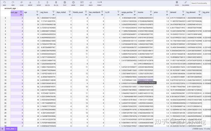
train_data.head()
train_data.describe()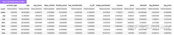

查看数据:

## 变量转换
## 结果变量 target
train_data["log_demand"] = np.log(train_data
["demand"])
train_data["log_price"] = np.log(train_data["price"])
Y = train_data["log_demand"].values ## from Series to np array
## 干预变量 treatment
T = train_data["log_price"].values
## 关键自变量
X = train_data[["income"]].values
## 混淆变量 - 控制变量
confounder_names = ["account_age", "age", "avg_hours", "days_visited", "friends_count", "has_membership", "is_US", "songs_purchased"]
W = train_data[confounder_names].values
## 构造关键自变量的测试数据
X_test = np.linspace(0, 5, 100).reshape(-1, 1)
X_test_data = pd.DataFrame(X_test, columns=["income"])2. DoWhy: 构建因果框架
## 初始化 EconML 估计器
est = LinearDML(model_y=GradientBoostingRegressor(), model_t=GradientBoostingRegressor(),
              featurizer=PolynomialFeatures(degree=2, include_bias=False))
## 通过 DoWhy 进行拟合
est_dw = est.dowhy.fit(Y, T, X=X, W=W, outcome_names=["log_demand"], treatment_names=["log_price"], feature_names=["income"],
               confounder_names=confounder_names, inference="statsmodels")
## 画出因果图
try:
    # Try pretty printing the graph. Requires pydot and pygraphviz
    display(
        Image(to_pydot(est_dw._graph._graph).create_png())
except:
    # Fall back on default graph view
est_dw.view_model() 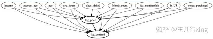

## 输出估计结果
identified_estimand = est_dw.identified_estimand_
print(identified_estimand)
[Out: ]
Estimand type: nonparametric-ate
### Estimand : 1
Estimand name: backdoor
Estimand expression:
────────────(Expectation(log_demand|friends_count,income,avg_hours,account_age
d[log_price]
,is_US,days_visited,age,has_membership,songs_purchased))
Estimand assumption 1, Unconfoundedness: If U→{log_price} and U→log_demand then P(log_demand|log_price,friends_count,income,avg_hours,account_age,is_US,days_visited,age,has_membership,songs_purchased,U) = P(log_demand|log_price,friends_count,income,avg_hours,account_age,is_US,days_visited,age,has_membership,songs_purchased)
### Estimand : 2
Estimand name: iv
No such variable found!
### Estimand : 3
Estimand name: frontdoor
No such variable found!
3. EconML: 估计因果效应
具体的估计模型如下(和计量中的中介效应在形式上有点相似)

## 基于真实的数据生成过程,估计因果效应
def gamma_fn(X):
return -3 - 14 * (X["income"] < 1)
def beta_fn(X):
return 20 + 0.5 * (X["avg_hours"]) + 5 * (X["days_visited"] > 4)
def demand_fn(data, T):
Y = gamma_fn(data) * T + beta_fn(data)
return Y
def true_te(x, n, stats):
if x < 1:
subdata = train_data[train_data["income"] < 1].sample(n=n, replace=True)
else:
subdata = train_data[train_data["income"] >= 1].sample(n=n, replace=True)
te_array = subdata["price"] * gamma_fn(subdata) / (subdata["demand"])
if stats == "mean":
return np.mean(te_array)
elif stats == "median":
return np.median(te_array)
elif isinstance(stats, int):
return np.percentile(te_array, stats)
## 估计结果和置信区间
truth_te_estimate = np.apply_along_axis(true_te, 1, X_test, 1000, "mean")
truth_te_upper = np.apply_along_axis(
true_te, 1, X_test, 1000, 95)
truth_te_lower = np.apply_along_axis(true_te, 1, X_test, 1000, 5) 接下来,对估计的结果和真实情况进行对比:
plt.figure(figsize=(16, 10))
plt.plot(X_test.flatten(), te_pred, label="Sales Elasticity Prediction")
plt.plot(X_test.flatten(), truth_te_estimate, "--", label="True Elasticity")
plt.fill_between(
    X_test.flatten(),
    te_pred_interval[0].flatten(),
    te_pred_interval[1].flatten(),
    alpha=0.2,
    label="95% Confidence Interval",
plt.fill_between(
    X_test.flatten(),
    truth_te_lower,
    truth_te_upper,
    alpha=0.2,
    label="True Elasticity Range",
plt.xlabel("Income")
plt.ylabel("Songs Sales Elasticity")
plt.title("Songs Sales Elasticity vs Income")
plt.legend(loc="lower right")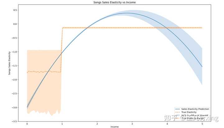

上图解读:
- 真实的干预效果非线性(橘色虚线)
- 拟合的模型基于 income 的二次项(且二次项的系数为负,抛物线开口向下)
- 不管是真实还是拟合的结果都能看出,收入低弹性高,收入高弹性低(这好像是个常识?)
查看具体的估计结果系数:
## 显示X和截距项的估计结果信息
est_dw.summary(feature_names=["income"])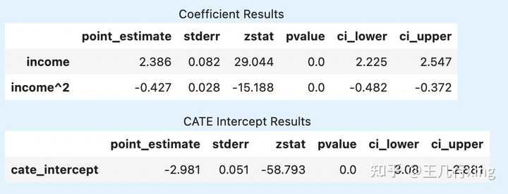

非参估计与HTE: CausalForestDML
前面的估计我们使用了线性的模型,发现估计效果整体虽然还行,但是离真实情况仍有显著差距。这里我们转向非参估计,基于因果森林重新对数据进行建模和拟合。
## 初始化
est_nonparam = CausalForestDML(model_y=GradientBoostingRegressor(), model_t=GradientBoostingRegressor())
## 通过 DoWhy 进行拟合
est_nonparam_dw = est_nonparam.dowhy.fit(Y, T, X=X, W=W, outcome_names=["log_demand"], treatment_names=["log_price"],
                                         feature_names=["income"], confounder_names=confounder_names, inference="blb")
## 计算干预效应及其置信区间
te_pred = est_nonparam_dw.effect(X_test).flatten()
te_pred_interval = est_nonparam_dw.effect_interval(X_test)
## 比较非参估计的结果和真实结果
plt.figure(figsize=(16, 10))
plt.plot(X_test.flatten(), te_pred, label="Sales Elasticity Prediction")
plt.plot(X_test.flatten(), truth_te_estimate, "--", label="True Elasticity")
plt.fill_between(
    X_test.flatten(),
    te_pred_interval[0].flatten(),
    te_pred_interval[1].flatten(),
    alpha=0.2,
    label="95% Confidence Interval",
plt.fill_between(
    X_test.flatten(),
    truth_te_lower,
    truth_te_upper,
    alpha=0.2,
    label="True Elasticity Range",
plt.xlabel("Income")
plt.ylabel("Songs Sales Elasticity")
plt.title("Songs Sales Elasticity vs Income")
plt.legend(loc="lower right")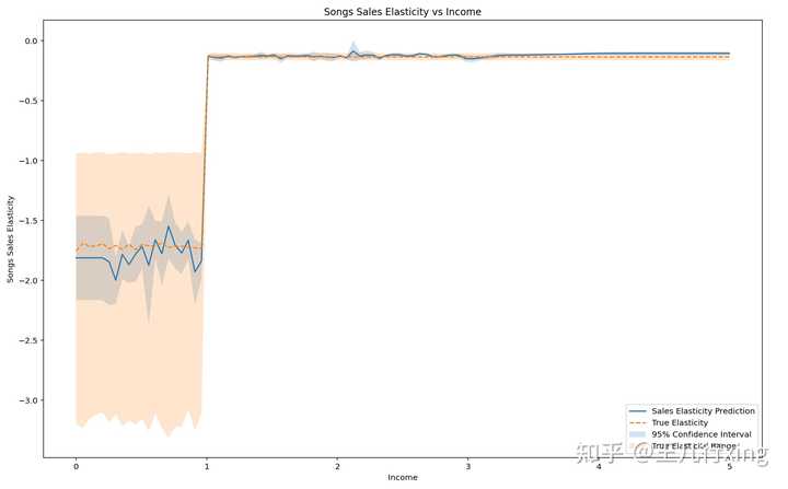

上图解读:
- 拟合效果远好过线性模型(LinearDML)
- 估计结果置信区间完全覆盖真实情况
- 同样的,估计结果显示收入低弹性高,收入高弹性低
4. DoWhy:稳健性检验
4.1 加入一个随机的共同原因变量
res_random = est_nonparam_dw.refute_estimate(method_name="random_common_cause")
print(res_random)
[Out: ]
Refute: Add a Random Common Cause
Estimated effect:-0.9561140448923923
New effect:-0.963688374616349
结果解读:点估计结果变化不大。
4.2 加入一个无法观测到的的共同原因变量
res_unobserved = est_nonparam_dw.refute_estimate(
    method_name="add_unobserved_common_cause",
    confounders_effect_on_treatment="linear",
    confounders_effect_on_outcome="linear",
    effect_strength_on_treatment=0.1,
    effect_strength_on_outcome=0.1,
print(res_unobserved)
[Out: ]
Refute: Add an Unobserved Common Cause
Estimated effect:-0.9561140448923923
New effect:0.1932125423770007
结果解读:点估计结果变化较大,但是仍然不等于0?(这里为什么不显示p值?)。
4.3 安慰剂检验
这里所谓安慰剂检验,就是把干预变量(价格)替换成一个噪音变量,理想的结果是估计的系数接近于,或者p值不显著。
res_placebo = est_nonparam_dw.refute_estimate(
    method_name="placebo_treatment_refuter", placebo_type="permute",
    num_simulations=3
print(res_placebo)
[Out: ]
Refute: Use a Placebo Treatment
Estimated effect:-0.9561140448923923
New effect:-0.00769355893605958
p value:0.21924855198612314
解读:点估计的结果变化较大,且p值不在显著。(难道是如果显著就不显示p值?)
4.5 随机删除部分数据
res_subset = est_nonparam_dw.refute_estimate(
    method_name="data_subset_refuter", subset_fraction=0.8,
    num_simulations=3)
print(res_subset)
Refute: Use a subset of data
Estimated effect:-0.9561140448923923
New effect:-0.957908388178223
p value:0.022684332959365117
估计结果相差不大,并且显著(显示了p值!)
5. EconML:干预的异质性
intrp = SingleTreeCateInterpreter(include_model_uncertainty=True, max_depth=2, min_samples_leaf=10)
intrp.interpret(est_nonparam_dw, X_test)
plt.figure(figsize=(25, 5))
intrp.plot(feature_names=["income"], fontsize=12)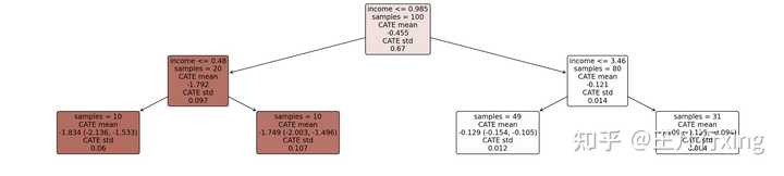

结果解读:左边深色区域表示价格弹性较大,右边结果显示较小,即对打折的反应是不同的。
5.1 SingleTreePolicyInterpreter: CATE 模型的解释
intrp = SingleTreePolicyInterpreter(risk_level=0.05, max_depth=2, min_samples_leaf=1, min_impurity_decrease=0.001)
intrp.interpret(est_nonparam_dw, X_test, sample_treatment_costs=-1)
plt.figure(figsize=(25, 5))
intrp.plot(feature_names=["income"], treatment_names=["Discount", "No-Discount"], fontsize=12)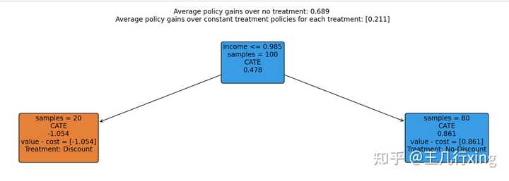

5.2 比较不同的打折策略
## 定义折扣策略收益函数
def revenue_fn(data, discount_level1, discount_level2, baseline_T, policy):
    policy_price = baseline_T * (1 - discount_level1) * policy + baseline_T * (1 - discount_level2) * (1 - policy)
    demand = demand_fn(data, policy_price)
    rev = demand * policy_price
    return rev
policy_dic = {}
## 本文的策略
policy = intrp.treat(X)
policy_dic["Our Policy"] = np.mean(revenue_fn(train_data, 0, 0.1, 1, policy))
## 原始策略
policy_dic["Previous Strategy"] = np.mean(train_data["price"] * train_data["demand"])
## 对所有人都打折
policy_dic["Give Everyone Discount"] = np.mean(revenue_fn(train_data, 0.1, 0, 1, np.ones(len(X))))
## 对所有人都不打折
policy_dic["Give No One Discount"] = np.mean(revenue_fn(train_data, 0, 0.1, 1, np.ones(len(X))))
## 对穷人打折,对富人涨价