【论文翻译】SoundStream: An End-to-End Neural Audio Codec

1 INTRODUCTION
Audio codecs can be partitioned into two broad categories: waveform codecs and parametric codecs .
Waveform codecs aim at producing at the decoder side a faithful reconstruction of the input audio samples.
In most cases, these codecs rely on transform coding techniques: a (usually invertible) transform is used to map an input time-domain waveform to the time-frequency domain. Then, transform coefficients are quantized and entropy coded.
At the decoder side the transform is inverted to reconstruct a time-domain waveform.
Often the bit allocation at the encoder is driven by a perceptual model, which determines the quantization process.
Generally, waveform codecs make little or no assumptions about the type of audio content and can thus operate on general audio. As a consequence of this, they produce very high-quality audio at medium-to-high bitrates, but they tend to introduce coding artifacts when operating at low bitrates.
Parametric codecs aim at overcoming this problem by making specific assumptions about the source audio to be encoded (in most cases, speech) and introducing strong priors in the form of a parametric model that describes the audio synthesis process.
The encoder estimates the parameters of the model, which are then quantized.
The decoder generates a time-domain waveform using a synthesis model driven by quantized parameters.
Unlike waveform codecs, the goal is not to obtain a faithful reconstruction on a sample-by-sample basis, but rather to generate audio that is perceptually similar to the original.
音频编解码器可分为两大类: 波形编解码器 和 参数编解码器 。
波形编解码器旨在在解码器端对输入音频样本进行忠实的重建。
在大多数情况下,这些编解码器依赖于变换编码技术:(通常是可逆的)变换用于将输入时域波形映射到时频域。 然后,对变换系数进行量化和熵编码。
在解码器端,变换被反转以重建时域波形。
通常,编码器的比特分配是由感知模型驱动的,它决定了量化过程。
一般而言,波形编解码器对音频内容的类型做出很少或根本没有假设,因此可以对一般音频进行操作。因此,它们可以以中高比特率生成非常高质量的音频,但在以低比特率运行时往往会引入编码伪像。
参数编解码器旨在通过对要编码的源音频(在大多数情况下是语音)做出特定假设并以描述音频合成过程的参数模型的形式引入强先验来克服这个问题。
编码器估计模型的参数,然后对其进行量化。
解码器使用由量化参数驱动的合成模型生成时域波形。
与波形编解码器不同,目标不是在逐个样本的基础上获得忠实的重建,而是生成在感知上与原始音频相似的音频。
Traditional waveform and parametric codecs rely on signal processing pipelines and carefully engineered design choices, which exploit in-domain knowledge on psycho-acoustics and speech synthesis to improve coding efficiency.
More recently machine learning models have been successfully applied in the field of audio compression, demonstrating the additional value brought by data-driven solutions.
For example, it is possible to apply them as a post-processing step to improve the quality of existing codecs.
This can be accomplished either via audio superresolution, i.e., extending the frequency bandwidth [1], via audio denoising, i.e., removing lossy coding artifacts [2], or via packet loss concealment
传统的波形和参数编解码器依赖于信号处理管道和精心设计的设计选择,它们利用心理声学和语音合成领域的知识来提高编码效率。
最近,机器学习模型已成功应用于音频压缩领域,展示了数据驱动解决方案带来的附加价值。
例如,可以将它们用作后处理步骤以提高现有编解码器的质量。
这可以通过音频超分辨率,即扩展频率带宽 [1],通过音频降噪,即去除有损编码伪影 [2],或通过数据包丢失隐藏来实现。
Other solutions adopt ML-based models as an integral part of the audio codec architecture.
In these areas, recent advances in text-to-speech (TTS) technology proved to be a key ingredient.
For example, WaveNet [4], a strong generative model originally applied to generate speech from text, was adopted as a decoder in a neural codec [5], [6].
Other neural audio codecs adopt different model architectures, e.g., WaveRNN in LPCNet [7] and WaveGRU in Lyra [8], all targeting speech at low bitrates.
其他解决方案采用基于 ML 的模型作为音频编解码器架构的组成部分。
在这些领域,文本转语音 (TTS) 技术的最新进展被证明是一个关键因素。
例如,WaveNet是一种强大的生成模型,最初用于从文本生成语音,在神经编解码器被用作解码器。
其他神经音频编解码器采用不同的模型架构,例如 LPCNet中的 WaveRNN 和 Lyra中的 WaveGRU,均以低比特率语音为目标。
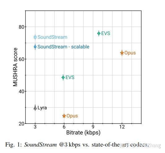

In this paper we propose SoundStream, a novel audio codec that can compress speech, music and general audio more efficiently than previous codecs, as illustrated in Figure 1.
SoundStream leverages state-of-the-art solutions in the field of neural audio synthesis, and introduces a new learnable quantization module, to deliver audio at high perceptual quality, while operating at low-to-medium bitrates.
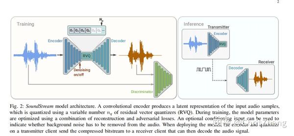
Figure 2 illustrates the high level model architecture of the codec. A fully convolutional encoder receives as input a time-domain waveform and produces a sequence of embeddings at a lower sampling rate, which are quantized by a residual vector quantizer.
A fully convolutional decoder receives the quantized embeddings and reconstructs an approximation of the original waveform.
The model is trained end-to-end using both reconstruction and adversarial losses.
To this end, one (or more) discriminators are trained jointly, with the goal of distinguishing the decoded audio from the original audio and, as a by-product, provide a space where a feature-based reconstruction loss can be computed.
Both the encoder and the decoder only use causal convolutions, so the overall architectural latency of the model is determined solely by the temporal resampling ratio between the original time-domain waveform and the embeddings.
在本文中,我们提出了 SoundStream,这是一种新颖的音频编解码器,可以比以前的编解码器更有效地压缩语音、音乐和一般音频,如图 1 所示。
SoundStream 利用在神经网络音频合成领域最先进的解决方案,并引入了一个新的可学习量化模块,以提供高感知质量的音频,同时以中低比特率运行。
图 2 说明了编解码器的高级模型架构。 全卷积编码器接收时域波形作为输入,并以较低的采样率生成一系列嵌入,这些嵌入由残差向量量化器量化。
全卷积解码器接收量化嵌入并重建原始波形的近似值。
该模型使用重建和对抗性损失进行端到端训练。
为此,联合训练一个(或多个)鉴别器,目的是将解码后的音频与原始音频区分开来,并作为副产品提供一个可以计算基于特征的重建损失的空间。
编码器和解码器都只使用因果卷积,因此模型的整体架构延迟完全取决于原始时域波形和嵌入之间的时间重采样率。

In summary, this paper makes the following key contributions:
• We propose SoundStream, a neural audio codec in which all the constituent components (encoder, decoder and quantizer) are trained end-to-end with a mix of reconstruction and adversarial losses to achieve superior audio quality.
• We introduce a new residual vector quantizer, and investigate the rate-distortion-complexity trade-offs implied by its design. In addition, we propose a novel “quantizer dropout” technique for training the residual vector quantizer, which enables a single model to handle different bitrates.
• We demonstrate that learning the encoder brings a very significant coding efficiency improvement, with respect to a solution that adopts mel-spectrogram features.
• We demonstrate by means of subjective quality metrics that SoundStream outperforms both Opus and EVS over a wide range of bitrates.
• We design our model to support streamable inference, which can operate at low-latency. When deployed on a smartphone, it runs in real-time on a single CPU thread.
• We propose a variant of the SoundStream codec that performs jointly audio compression and enhancement, without introducing additional latency.
总之,本文做出以下主要贡献:
• 我们提出了 SoundStream,这是一种神经音频编解码器,其中所有组成部分(编码器、解码器和量化器)都经过端到端的训练,混合了重建和对抗性损失,以实现卓越的音频质量。
• 我们引入了一种新的残差向量量化器,并研究了其设计所隐含的速率-失真-复杂性权衡。 此外,我们提出了一种新的“量化器丢失”技术来训练残差向量量化器,使单个模型能够处理不同的比特率。
• 我们证明,相对于采用梅尔谱图特征的解决方案,学习编码器带来了非常显着的编码效率改进。
• 我们通过主观质量指标证明,SoundStream 在广泛的比特率范围内优于 Opus 和 EVS。
• 我们设计我们的模型以支持可在低延迟下运行的流式推理。 当部署在智能手机上时,它会在单个 CPU 线程上实时运行。
• 我们提出了一种 SoundStream 编解码器的变体,它可以联合执行音频压缩和增强,而不会引入额外的延迟。
2 RELATED WORK
Traditional audio codecs
Opus [9] and EVS [10] are state-of-the-art audio codecs, which combine traditional coding tools, such as LPC, CELP and MDCT, to deliver high coding efficiency over different content types, bitrates and sampling rates, while ensuring low-latency for real-time audio communications. We compare SoundStream with both Opus and EVS in our subjective evaluation.
传统语音编解码器
Opus 和 EVS 是最先进的音频编解码器,它们结合了传统的编码工具,如 LPC、CELP 和 MDCT,可在不同的内容类型、比特率和采样率下提供高编码效率,同时确保实时音频通信的低延迟。 我们在主观评价中将 SoundStream 与 Opus 和 EVS 进行了比较。
Audio generative models
Several generative models have been developed for converting text or coded features into audio waveforms.
WaveNet [4] allows for global and local signal conditioning to synthesize both speech and music.
SampleRNN [11] uses recurrent networks in a similar fashion, but it relies on previous samples at different scales.
These auto-regressive models deliver very high-quality audio, at the cost of increased computational complexity, since samples are generated one by one.
To overcome this issue, Parallel WaveNet [12] allows for parallel computation, yielding considerable speedup during inference.
Other approaches involve lightweight and sparse models [13] and networks mimicking the fast Fourier transform as part of the model [7], [14].
More recently, generative adversarial models have emerged as a solution able to deliver high-quality audio with a lower computational complexity.
MelGAN [15] is trained to produce audio waveforms when conditioned on mel-spectrograms, training a multi-scale waveform discriminator together with the generator.
HiFiGAN [16] takes a similar approach but it applies discriminators to both multiple scales and multiple periods of the audio samples.
The design of the decoder and the losses in SoundStream is based on this class of audio generative models.
已经开发了几种生成模型,用于将文本或编码特征转换为音频波形。
WaveNet [4] 允许全局和局部信号调节以合成语音和音乐。
SampleRNN [11] 以类似的方式使用循环网络,但它依赖于不同规模的先前样本。
这些自回归模型以增加计算复杂性为代价提供非常高质量的音频,因为样本是一个一个生成的。
为了克服这个问题,Parallel WaveNet [12] 允许并行计算,在推理过程中产生相当大的加速。
其他方法涉及轻量级和稀疏模型 [13] 以及模仿快速傅里叶变换的网络作为模型的一部分 [7],[14]。
最近,生成对抗模型已经成为一种能够以较低的计算复杂性提供高质量音频的解决方案。
MelGAN [15] 被训练在以梅尔频谱图为条件时产生音频波形,与发生器一起训练多尺度波形鉴别器。
HiFiGAN [16] 采用了类似的方法,但它将鉴别器应用于音频样本的多个尺度和多个周期。
SoundStream中decoder和loss的设计都是基于这类音频生成模型。
Audio enhancement
Deep neural networks have been applied to different audio enhancement tasks, ranging from denoising [17]–[21] to dereverberation [22], [23], lossy coding denoising [2] and frequency bandwidth extension [1], [24].
In this paper we show that it is possible to jointly perform audio enhancement and compression with a single model, without introducing additional latency.
深度神经网络已应用于不同的音频增强任务,从去噪 [17]-[21] 到去混响 [22]、[23]、有损编码去噪 [2] 和频率带宽扩展 [1]、[24]。
在本文中,我们展示了可以使用单个模型联合执行音频增强和压缩,而不会引入额外的延迟。
Vector quantization
Learning the optimal quantizer is a key element to achieve high coding efficiency.
Optimal scalar quantization based on Lloyd’s algorithm [25] can be extended to a high-dimensional space via the generalized Lloyd algorithm (GLA) [26], which is very similar to k-means clustering [27].
In vector quantization [28], a point in a high-dimensional space is mapped onto a discrete set of code vectors.
Vector quantization has been commonly used as a building block of traditional audio codecs [29].
For example, CELP [30] adopts an excitation signal encoded via a vector quantizer codebook.
More recently, vector quantization has been applied in the context of neural network models to compress the latent representation of input features.
For example, in variational autoencoders, vector quantization has been used to generate images [31], [32] and music [33], [34].
Vector quantization can become prohibitively expensive, as the size of the codebook grows exponentially when rate is increased.
For this reason, structured vector quantizers [35], [36] (e.g., residual, product, lattice vector quantizers, etc.) have been proposed to obtain a trade-off between computational complexity and coding efficiency in traditional codecs.
In SoundStream, we extend the learnable vector quantizer of VQ-VAE [31] and introduce a residual (a.k.a. multi-stage) vector quantizer, which is learned end-to-end with the rest of the model.
To the best of the authors knowledge, this is the first time that this form of vector quantization is used in the context of neural networks and trained end-to-end with the rest of the model.
可学习最佳量化器是实现高编码效率的关键因素。
基于Lloyd算法 [25] 的最优标量量化可以通过广义Lloyd算法 (GLA) [26] 扩展到高维空间,这与 k 均值聚类 [27] 非常相似。
在向量量化 [28] 中,高维空间中的一个点被映射到一组离散的代码向量上。
向量量化通常用作传统音频编解码器的构建块 [29]。
例如,CELP [30] 采用通过向量量化码本编码的激励信号。
最近,向量量化已应用于神经网络模型的上下文中,以压缩输入特征的潜在表示。
例如,在变分自动编码器中,向量量化已被用于生成图像 [31]、[32] 和音乐 [33]、[34]。
向量量化可能变得非常昂贵,因为码本的大小在速率增加时呈指数增长。
出于这个原因,已经提出了结构化向量量化器 [35]、[36](例如,残差、乘积、格向量量化器等),以在传统编解码器中获得计算复杂性和编码效率之间的权衡。
在 SoundStream 中,我们扩展了 VQ-VAE [31] 的可学习向量量化器并引入了一个残差(又名多级)向量量化器,它与模型的其余部分一起端到端学习。
据作者所知,这是第一次在神经网络环境中使用这种形式的向量量化,并与模型的其余部分进行端到端训练。
Neural audio codecs
End-to-end neural audio codecs rely on data-driven methods to learn efficient audio representations, instead of relying on handcrafted signal processing components.
Autoencoder networks with quantization of hidden features were applied to speech coding early on [37].
More recently, a more sophisticated deep convolutional network for speech compression was described in [38].
Efficient compression of audio using neural networks has been demonstrated in several works, mostly targeting speech coding at low bitrates.
A VQ-VAE speech codec was proposed in [6], operating at 1.6 kbps.
Lyra [8] is a generative model that encodes quantized mel-spectrogram features of speech, which are decoded with an auto-regressive WaveGRU model to achieve state-of-the-art results at 3 kbps.
A very low-bitrate codec was proposed in [39] by decoding speech representations obtained via self-supervised learning.
An end-to-end audio codec targeting general audio at high bitrates (i.e., above 64 kbps) was proposed in [40].
The model architecture adopts a residual coding pipeline, which consists of multiple autoencoding modules and a psycho-acoustic model is used to drive the loss function during training.
端到端神经音频编解码器依靠数据驱动的方法来学习高效的音频表示,而不是依赖手工制作的信号处理组件。
具有隐藏特征量化的自动编码器网络很早就被应用于语音编码 [37]。
最近,[38] 中描述了一种用于语音压缩的更复杂的深度卷积网络。
使用神经网络对音频进行高效压缩已在多项工作中得到证明,主要针对低比特率的语音编码。
[6] 中提出了一种 VQ-VAE 语音编解码器,以 1.6 kbps 的速度运行。
Lyra [8] 是一种生成模型,它对语音的量化梅尔谱图特征进行编码,并使用自回归 WaveGRU 模型对其进行解码,以 3 kbps 的速度获得最先进的结果。
[39] 中提出了一种非常低比特率的编解码器,通过解码通过自监督学习获得的语音表示。
[40] 中提出了一种针对高比特率(即高于 64 kbps)的通用音频的端到端音频编解码器。
该模型架构采用残差编码流水线,由多个自动编码模块组成,并使用心理声学模型来驱动训练过程中的损失函数。
Unlike [39] which specifically targets speech by combining speaker, phonetic and pitch embeddings, SoundStream does not make assumptions on the nature of the signal it encodes, and thus works for diverse audio content types.
While [8] learns a decoder on fixed features, SoundStream is trained in an end-to-end fashion.
Our experiments (see Section IV) show that learning the encoder increases the audio quality substantially.
SoundStream achieves bitrate scalability, i.e., the ability of a single model to operate at different bitrates at no additional cost, thanks to its residual vector quantizer and to our original quantizer dropout training scheme (see Section III-C).
This is unlike [38] and [40] which enforce a specific bitrate during training and require training a different model for each target bitrate.
A single SoundStream model is able to compress speech, music and general audio, while operating at a 24 kHz sampling rate and low-to-medium bitrates (3 kbps to 18 kbps in our experiments), in real time on a smartphone CPU.
This is the first time that a neural audio codec is shown to outperform state-of-the-art codecs like Opus and EVS over this broad range of bitrates.
与 [39] 通过结合说话人、语音和音调嵌入专门针对语音不同,SoundStream 不对其编码的信号的性质做出假设,因此适用于不同的音频内容类型。
[8] 在固定特征上学习解码器,而 SoundStream 则以端到端的方式进行训练。
我们的实验(参见第 IV 节)表明,学习编码器可以显着提高音频质量。
SoundStream 实现了比特率可扩展性,即单个模型无需额外成本即可在不同比特率下运行的能力,这要归功于其残差向量量化器和我们最初的量化器丢失训练方案(参见第 III-C 节)。
这与 [38] 和 [40] 不同,后者在训练期间强制执行特定的比特率,并需要为每个目标比特率训练不同的模型。
单个 SoundStream 模型能够压缩语音、音乐和一般音频,同时在智能手机 CPU 上以 24 kHz 采样率和中低比特率(在我们的实验中为 3 kbps 至 18 kbps)实时运行。
这是神经音频编解码器首次显示出在如此广泛的比特率范围内优于 Opus 和 EVS 等最先进的编解码器。
Joint compression and enhancement
Recent work has explored joint compression and enhancement.
The work in [41] trains a speech enhancement system with a quantized bottleneck.
Instead, SoundStream integrates a time-dependent conditioning layer, which allows for real-time controllable denoising.
As we design SoundStream as a general-purpose audio codec, controlling when to denoise allows for encoding acoustic scenes and natural sounds that would be otherwise removed.
最近的工作探索了压缩和增强联合在一起的方式。
[41] 中的工作训练了一个具有量化瓶颈的语音增强系统。
相反,SoundStream 集成了一个时间相关的调节层,它允许实时可控的降噪。
当我们将 SoundStream 设计为通用音频编解码器时,控制何时去噪允许对原本会被移除的声学场景和自然声音进行编码。
3. Model
We consider a single channel recording x ∈ R^T , sampled at f_s .
The SoundStream model consists of a sequence of three building blocks, as illustrated in Figure 2:
• an encoder, which maps x to a sequence of embeddings(see Section III-A),
• a residual vector quantizer, which replaces each embedding by the sum of vectors from a set of finite codebooks, thus compressing the representation with a target number of bits (see Section III-C),
• a decoder, which produces a lossy reconstruction xˆ ∈ RT from quantized embeddings (see Section III-B).
The model is trained end-to-end together with a discriminator (see Section III-D), using the mix of adversarial and reconstruction losses described in Section III-E.
Optionally, a conditioning signal can be added, which determines whether denoising is applied at the encoder or decoder side, as detailed in Section III-F.
我们考虑在 f_s 采样的单通道记录 x ∈ R^T 。
SoundStream 模型由一系列三个构建块组成,如图 2 所示:
• 编码器,将 x 映射到嵌入序列(参见第 III-A 节),
• 残差向量量化器,用一组有限码本的向量总和代替每个嵌入,从而用目标位数压缩表示(见第 III-C 节),
• 一个解码器,它从量化的嵌入中产生有损重建 \tilde{x} ∈ R^T (见第 III-B 节)。
该模型与鉴别器一起进行端到端训练(参见第 III-D 节),使用第 III-E 节中描述的对抗性和重建损失的组合。
可选地,可以添加一个调节信号,它决定是在编码器还是解码器端应用去噪,如第 III-F 节中详述。
A. Encoder architecture
The encoder architecture is illustrated in Figure 3 and follows the same structure as the streaming SEANet encoder described in [1], but without skip connections. It consists of a 1D convolution layer (with C_{enc} channels), followed by B_{enc} convolution blocks. Each of the blocks consists of three residual units, containing dilated convolutions with dilation rates of 1, 3, and 9, respectively, followed by a down-sampling layer in the form of a strided convolution.
The number of channels is doubled whenever down-sampling, starting from Cenc.
A final 1D convolution layer with a kernel of length 3 and a stride of 1 is used to set the dimensionality of the embeddings to D.
To guarantee real-time inference, all convolutions are causal. This means that padding is only applied to the past but not the future in both training and offline inference, whereas no padding is used in streaming inference.
We use the ELU activation [42]and we do not apply any normalization.
The number Benc of convolution blocks and the corresponding striding sequence determines the temporal resampling ratio between the input waveform and the embeddings.
For example, when Benc = 4 and using (2, 4, 5, 8) as strides, one embedding is computed every M = 2 · 4 · 5 · 8 = 320 input samples.
Thus, the encoder outputs enc(x) ∈ R S×D, with S = T /M
编码器架构如图 3 所示,遵循与 [1] 中描述的流式 SEANet 编码器相同的结构,但没有跳过连接。 它由一维卷积层(带有 C_{enc} 通道)和 B_{enc} 卷积块组成。 每个块由三个残差单元组成,包含扩张率分别为 1、3 和 9 的扩张卷积,后跟一个跨步卷积形式的下采样层。
从 C_{enc} 开始,每当下采样时,通道数都会加倍。
最后一个 1D 卷积层,内核长度为 3,步长为 1,用于将嵌入的维数设置为 D。
为了保证实时推理,所有的卷积都是因果关系。 这意味着在训练和离线推理中填充仅适用于过去而不适用于未来,而在流式推理中不使用填充。
我们使用 ELU 激活 [42],我们不应用任何归一化。
卷积块的数量 B_{enc} 和相应的跨步序列决定了输入波形和嵌入之间的时间重采样率。
例如,当 B_{enc} = 4 并使用 (2, 4, 5, 8) 作为步长时,每 M = 2 · 4 · 5 · 8 = 320 个输入样本计算一个嵌入。
因此,编码器输出 enc(x) ∈ R^{S×D} ,其中 S = T /M
B. Decoder architecture
The decoder architecture follows a similar design, as illustrated in Figure 3.
A 1D convolution layer is followed by a sequence of B_{dec} convolution blocks.
The decoder block mirrors the encoder block, and consists of a transposed convolution for up-sampling followed by the same three residual units.
We use the same strides as the encoder, but in reverse order, to reconstruct a waveform with the same resolution as the input waveform.
The number of channels is halved whenever upsampling, so that the last decoder block outputs Cdec channels.
A final 1D convolution layer with one filter, a kernel of size 7 and stride 1 projects the embeddings back to the waveform domain to produce xˆ.
In Figure 3, the same number of channels in both the encoder and the decoder is controlled by the same parameter, i.e., C_{enc} = C_{dec} = C . We also investigate cases in which C_{enc} \ne C_{dec} , which results in a computationally lighter encoder and a heavier decoder, or vice-versa (see Section V-D).
解码器架构遵循类似的设计,如图 3 所示。
一维卷积层之后是一系列 B_{dec} 卷积块。
解码器块反映了编码器块,由用于上采样的转置卷积和后跟相同的三个残差单元组成。
我们使用与编码器相同的步幅,但顺序相反,以重建与输入波形具有相同分辨率的波形。
每当上采样时通道数减半,因此最后一个解码器块输出 C_{dec} 通道。
带有一个滤波器、大小为 7 和步长为 1 的核的最终一维卷积层将嵌入投影回波形域以产生 x^。
在图 3 中,编码器和解码器中相同数量的通道由相同的参数控制,即 C_{enc} = C_{dec} = C 。我们还研究了 C_{enc} \ne C_{dec} 的情况,这导致计算更轻的编码器和 较重的解码器,反之亦然(参见第 V-D 节)。
C. Residual Vector Quantizer
The goal of the quantizer is to compress the output of the encoder enc(x) to a target bitrate R, expressed in bits/second (bps). In order to train SoundStream in an endto-end fashion, the quantizer needs to be jointly trained with the encoder and the decoder by backpropagation.
The vector quantizer (VQ) proposed in [31], [32] in the context of VQ-VAEs meets this requirement.
This vector quantizer learns a codebook of N vectors to encode each D-dimensional frame of enc(x).
The encoded audio enc(x) ∈ R^{S×D} is then mapped to a sequence of one-hot vectors of shape S × N, which can be represented using S log_2 N bits.
量化器的目标是将编码器 enc(x) 的输出压缩到目标比特率 R,以比特/秒 (bps) 表示。 为了以端到端的方式训练 SoundStream,量化器需要通过反向传播与编码器和解码器联合训练。
在 VQ-VAE 的背景下,[31]、[32] 中提出的向量量化器 (VQ) 满足了这一要求。
这个向量量化器学习一个 N 个向量的码本来编码 enc(x) 的每个 D 维帧。
然后将编码后的音频 enc(x) ∈ R^{S×D} 映射到形状为 S × N 的单热向量序列,可以使用 S log_2 N 位表示。
Limitations of Vector Quantization
As a concrete example, let us consider a codec targeting a bitrate R = 6000 bps.
When using a striding factor M = 320, each second of audio at sampling rate fs = 24000 Hz is represented by S = 75 frames at the output of the encoder.
This corresponds to r = 6000/75 = 80 bits allocated to each frame.
Using a plain vector quantizer, this requires storing a codebook with N = 280 vectors, which is obviously unfeasible.
作为一个具体示例,让我们考虑一个目标比特率 R = 6000 bps 的编解码器。
当使用跨步因子 M = 320 时,每秒采样率 fs = 24000 Hz 的音频在编码器的输出端由 S = 75 帧表示。
这对应于分配给每个帧的 r = 6000/75 = 80 位。
使用普通向量量化器,这需要存储一个包含 N = 280 个向量的码本,这显然是不可行的。
Residual Vector Quantizer
To address this issue we adopt a Residual Vector Quantizer (a.k.a. multi-stage vector quantizer [36]), which cascades Nq layers of VQ as follows.
The unquantized input vector is passed through a first VQ and quantization residuals are computed.
The residuals are then iteratively quantized by a sequence of additional Nq −1 vector quantizers, as described in Algorithm 1.
The total rate budget is uniformly allocated to each VQ, i.e., ri = r/Nq = log2 N.
For example, when using Nq = 8, each quantizer uses a codebook of size N = 2r/Nq = 280/8 = 1024.
For a target rate budget r, the parameter Nq controls the tradeoff between computational complexity and coding efficiency, which we investigate in Section V-D.
为了解决这个问题,我们采用了残差向量量化器(又名多级向量量化器 [36]),它按如下方式级联 VQ 的 Nq 层。
未量化的输入向量通过第一个 VQ 并计算量化残差。
然后,如算法 1 中所述,残差由一系列额外的 Nq -1 个向量量化器迭代量化。
总速率预算统一分配给每个 VQ,即 ri = r/Nq = log2 N。
例如,当使用 Nq = 8 时,每个量化器使用大小为 N = 2r/Nq = 280/8 = 1024 的码本。
对于目标速率预算 r,参数 Nq 控制计算复杂度和编码效率之间的权衡,我们在第 V-D 节中对此进行了研究。
The codebook of each quantizer is trained with exponential moving average updates, following the method proposed in VQ-VAE-2 [32].
To improve the usage of the codebooks we use two additional methods. First, instead of using a random initialization for the codebook vectors, we run the k-means algorithm on the first training batch and use the learned centroids as initialization.
This allows the codebook to be close to the distribution of its inputs and improves its usage.
Second, as proposed in [34], when a codebook vector has not been assigned any input frame for several batches, we replace it with an input frame randomly sampled within the current batch.
More precisely, we track the exponential moving average of the assignments to each vector (with a decay factor of 0.99) and replace the vectors of which this statistic falls below 2.
按照 VQ-VAE-2 中提出的方法,使用指数移动平均更新对每个量化器的码本进行训练。
为了改进密码本的使用,我们使用了两种额外的方法。 首先,我们没有对码本向量使用随机初始化,而是在第一个训练批次上运行 k-means 算法,并使用学习到的质心作为初始化。
这允许密码本接近其输入的分布并提高其使用率。
其次,如 [34] 中所提出的,当一个码本向量没有为几个批次分配任何输入帧时,我们将其替换为在当前批次中随机采样的输入帧。
更准确地说,我们跟踪分配给每个向量的指数移动平均值(衰减因子为 0.99),并替换该统计量低于 2 的向量。
Enabling bitrate scalability with quantizer dropout
Residual vector quantization provides a convenient framework for controlling the bitrate.
For a fixed size N of each codebook, the number of VQ layers Nq determines the bitrate.
Since the vector quantizers are trained jointly with the encoder/decoder, in principle a different SoundStream model should be trained for each target bitrate.
Instead, having a single bitrate scalable model that can operate at several target bitrates is much more practical, since this reduces the memory footprint needed to store model parameters both at the encoder and decoder side.
残差向量量化为控制比特率提供了一个方便的框架。
对于每个码本的固定大小 N,VQ 层数 Nq 决定了比特率。
由于向量量化器是与编码器/解码器联合训练的,原则上应该为每个目标比特率训练不同的 SoundStream 模型。
相反,拥有一个可以在多个目标比特率下运行的单一比特率可扩展模型更为实用,因为这减少了在编码器和解码器端存储模型参数所需的内存占用。
To train such a model, we modify Algorithm in the following way: for each input example, we sample n_q uniformly at random in [1; N_q] and only use quantizers Q_i for i = 1 . . . n_q .
This can be seen as a form of structured dropout [43] applied to quantization layers. Consequently, the model is trained to encode and decode audio for all target bitrates corresponding to the range nq = 1 . . . Nq. During inference, the value of nq is selected based on the desired bitrate.
Previous models for neural compression have relied on product quantization (wav2vec 2.0 [44]), or on concatenating the output of several VQ layers [5], [6]. With such approaches, changing the bitrate requires either changing the architecture of the encoder and/or the decoder, as the dimensionality changes, or retraining an appropriate codebook.
A key advantage of our residual vector quantizer is that the dimensionality of the embeddings does not change with the bitrate. Indeed, the additive composition of the outputs of each VQ layer progressively refines the quantized embeddings, while keeping the same shape. Hence, no architectural changes are needed in neither the encoder nor the decoder to accommodate different bitrates.
In Section V-C, we show that this method allows one to train a single SoundStream model, which matches the performance of models trained specifically for a given bitrate.
为了训练这样的模型,我们按以下方式修改 [1] :对于每个输入示例,我们在 [1; N_q] 中随机均匀采样 n_q , 并且只对 i = 1 . . n_q 使用量化器 Q_i 。
这可以看作是一种应用于量化层的结构化 dropout 形式。 因此,该模型被训练为对应于范围 1到 N_q 的所有目标比特率编码和解码音频。 在推理过程中, n_q 的值是根据所需的比特率选择的。
以前的神经压缩模型依赖于乘积量化 (wav2vec 2.0),或连接多个 VQ 层的输出。 使用此类方法,更改比特率需要随着维度的变化而更改编码器和/或解码器的架构,或者重新训练适当的码本。
我们的残差向量量化器的一个关键优势是嵌入的维数不随比特率变化。 事实上,每个 VQ 层的输出的加法组合逐渐细化量化嵌入,同时保持相同的形状。因此,编码器和解码器都不需要架构改变来适应不同的比特率。
在第V-C 节中,我们展示了这种方法允许训练单个 SoundStream 模型,该模型与专门针对给定比特率训练的模型的性能相匹配。
D. Discriminator architecture
To compute the adversarial losses described in Section III-E, we define two different discriminators:
i) a wave-based discriminator, which receives as input a single waveform;
ii) an STFT-based discriminator, which receives as input the complexvalued STFT of the input waveform, expressed in terms of real and imaginary parts.
Since both discriminators are fully convolutional, the number of logits in the output is proportional to the length of the input audio.
为了计算第 III-E 节中描述的对抗性损失,我们定义了两个不同的鉴别器:
i) 基于波的鉴别器,接收单个波形作为输入;
ii) 基于 STFT 的鉴别器,它接收输入波形的复值 STFT 作为输入,以实部和虚部表示。
由于两个鉴别器都是完全卷积的,因此输出中的逻辑数与输入音频的长度成正比。
For the wave-based discriminator, we use the same multi-resolution convolutional discriminator proposed in [15] and adopted in [45].
Three structurally identical models are applied to the input audio at different resolutions: original, 2-times down-sampled, and 4-times down-sampled.
Each single-scale discriminator consists of an initial plain convolution followed by four grouped convolutions, each of which has a group size of 4, a down-sampling factor of 4, and a channel multiplier of 4 up to a maximum of 1024 output channels.
They are followed by two more plain convolution layers to produce the final output, i.e., the logits.
对于基于波的鉴别器,我们使用在 [15] 中提出并在 [45] 中采用的相同多分辨率卷积鉴别器。
三种结构相同的模型应用于不同分辨率的输入音频:原始、2 倍下采样和 4 倍下采样。
每个单尺度鉴别器都包含一个初始普通卷积,然后是四个分组卷积,每个卷积的组大小为 4,下采样因子为 4,通道乘数为 4,最多 1024 个输出通道。
它们之后是两个更多的普通卷积层以产生最终输出,即 logits。
The STFT-based discriminator is illustrated in Figure 4 and operates on a single scale, computing the STFT with a window length of W = 1024 samples and a hop length of H = 256 samples. A 2D-convolution (with kernel size 7 × 7 and 32 channels) is followed by a sequence of residual blocks.
Each block starts with a 3×3 convolution, followed by a 3×4 or a 4×4 convolution, with strides equal to (1, 2) or (2, 2), where (st, sf ) indicates the down-sampling factor along the time axis and the frequency axis. We alternate between (1, 2) and (2, 2) strides, for a total of 6 residual blocks. The number of channels is progressively increased with the depth of the network.
At the output of the last residual block, the activations have shape
\frac {T} {(H · 2^3)} × \frac {F} {2^6}
, where T is the number of samples in the time domain and F = W/2 is the number of frequency bins.
The last layer aggregates the logits across the (down-sampled) frequency bins with a fully connected layer (implemented as a 1 × \frac{F} {2^6} convolution), to obtain a 1-dimensional signal in the (down-sampled) time domain.
基于 STFT 的鉴别器如图 4 所示,在单一尺度上运行,计算窗口长度 W = 1024 个样本和跳跃长度 H = 256 个样本的 STFT。 二维卷积(内核大小为 7 × 7 和 32 个通道)之后是一系列残差块。
每个块以 3×3 卷积开始,然后是 3×4 或 4×4 卷积,步长等于 (1, 2) 或 (2, 2),其中 (st, sf ) 表示下采样 沿时间轴和频率轴的因子。 我们在 (1, 2) 和 (2, 2) 步幅之间交替,总共有 6 个残差块。 通道的数量随着网络的深度逐渐增加。 在最后一个残差块的输出,激活有形状
\frac {T} {(H · 2^3)} × \frac {F} {2^6}
,其中 T 是时域中的样本数,F = W/2 是频率仓的数量。
最后一层使用全连接层(实现为 1 × \frac{F} {2^6} 卷积),以获得(下采样)时域中的一维信号。
参考
- ^ Real-time speech frequency bandwidth extension